
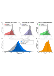
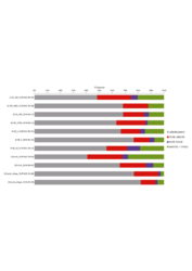
1 - Random forest results
Charts A, B and C compare the NMSE (Normalized Mean Square Error) distributions of real and randomized data. Chart D plots the distribution of paired differences between NMSEs obtained from the environmental (ENV) and original abundance (Operational Taxonomic Units, OTU) data (blue) versus ENV and randomized OTU data (gray). Chart E shows the AUC (Area under the curve) values of the binary classifiers obtained by thresholding the output of the regression model (class 0 associated to the 60% of the samples with the lowest OTU abundance and class 1 associated to the remaining 40%)
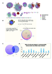
3 - Overview on the taxon network and its environmentally influenced edges
In (A), the 51 modules resulting from leading Eigenvector clustering (M.E.J. Newman, PNAS 103 (23):8577-8582, 2006) of the positively correlated taxon network are shown. The flow chart in (B) summarises taxon edge numbers for different analyses. From the 29,912 taxon edges that are part of environmental triplets, the 11,043 edges with significantly negative interaction information are considered as indirect (i.e. environmentally driven). Subsequent analyses were carried out on the remaining 81,590 taxon edges. The Venn diagram in (C) depicts the overlap between taxon edges that are part of environmental triplets, ocean-driven taxon edges and taxon edges classified as indirect. Finally, the bar chart in (D) plots the ratio between node percentages on phylum level in the 11,043 environmentally driven taxon edges (the indirect edges) versus the remaining edges. A ratio larger than one means that the percentage of the corresponding phylum is higher among the indirect taxon edges than in the remaining 81,590 taxon edges.

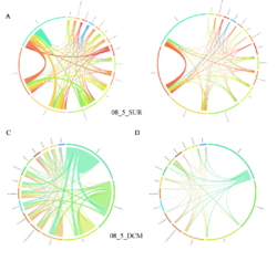
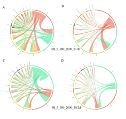
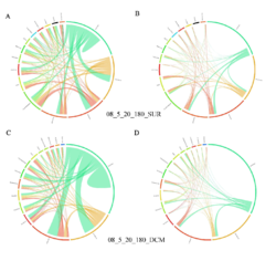
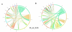
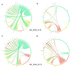
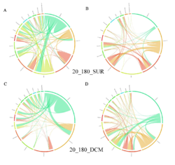
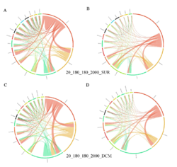
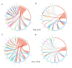
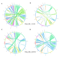
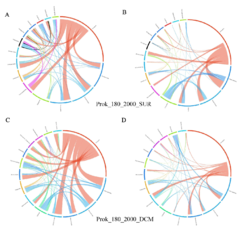
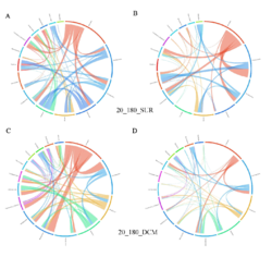
4 - Fraction- and layer-wise circos plots
Circos plot (M. Krzywinski et al., Genome Res 19:1639-1645, 2009) showing order-level copresences (left panels in each figure) and mutual exclusions (right panels in each figure) in individual fractions (08_5, 20_180, 180_2000 etc.) and layers (SUR: surface; DCM: deep chlorophyll maximum). For each plot, the band size for each taxon (labeled next to the bands) is proportional to the number of taxon edges; and the width of the ribbons is proportional to the numbers of copresence/mutual exclusions within (ribbons within one band) and between taxa (ribbons connecting two different bands)
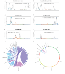
5 - Examples of ocean-specific correlated profiles
Examples of edges showing global copresence (A) and mutual exclusion patterns (B), as well as ocean specific edges for Mediterranean Sea, MS (C), South Pacific Ocean, SPO (D), Indian Ocean, IO (E) and Red Sea, RS (F). Operational taxonomic unit (OTU) abundances are colored by different oceans and the taxonomic assignment is printed alongside each OTU. The Southern Ocean (SO) has a distinct profile of region-specific edges that is dominated by bacterial taxa (G) instead of the common pattern observed across the entire network (H, plot conserving the scaffold of top connected taxa as in main Figure 2).
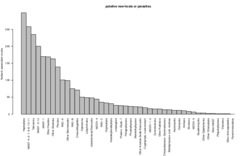
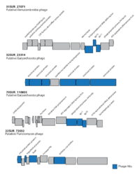
6 - Potential novel hosts and/or parasites
Parasites neighbors in large fractions. Parasites in large fractions may co-occur with their hosts or with (unknown) parasites. The distribution shows the taxonomic breakdown of the partners of parasites in the large fractions, from which all organisms that are known to host parasites is shown in main figure 3B.
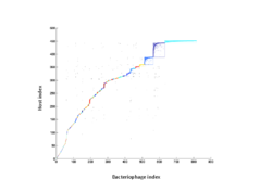
8 - Analysis of nestedness and modularity
Bacteriophage-host adjacency matrix re-arranged with BiMAT (Flores et al., arXiv:1406.6732v2 [q-bio.QM], 2014) to visualize modularity and nestedness. The adjacency matrix consists of positive associations between 816 bacteriophages and 451 hosts predicted for the surface and deep chlorophyll maximum layers.
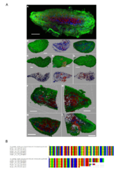
9 - Acoel flatworm microscopy images and alignment of V9 sequence
Confocal laser scanning microscope images of the acoel flatworm (in green) containing several microalgal cells intracellularly (red cells). Red, green, and blue fluorescence indicate the chlorophyll/plasts (autofluorescence), membranes (DiOC6), and DNA/nuclei (Hoechst33342), respectively. All the worm specimens that had been observed (>15) had displayed the endosymbiotic association with a microalgae (A-I). The lack of transparency of the worm and the low penetration of the DiOC6 dye did not permit to reveal the full cellular structure (membranes, nuclei and chloroplast) of the algae when localized inside the worm body. The algae nuclei signal is also very dim. Only the chlorophyll autofluorescence signal allows to discriminate the position of the algae inside the worm tissue (A, F-I). However when the epidermis of the worm is damaged (D), the unicellular structure and the integrity of the symbiont cells that are released from the cut becomes obvious. Sequence alignment of the V9 Tara-oceans metabarcode of the acoel flatworm from the predicted interaction (upper sequence) and six V9 sequences PCR amplified from six acoel flatworms found in station 22 that host symbiotic microalgae.
| Name | Size | Description | Download |
|---|---|---|---|
| W1 | 98K | Sample information | Download |
| W2 | 809K | Sample Environmental parameters | Download |
| W3 | 19K | Variation partitioning analysis | Download |
| W4 | 2.0M | Random forest results | Download |
| W5 | 38K | False discovery rate assessed with null models | Download |
| W6 | 36K | Network Properties | Download |
| W7 | 9.6M | The TARA ocean interactome | Download |
| W8 | 1.6M | Indirect edge detection results | Download |
| W9 | 2.3M | Reference interactions among eukaryotic plankton | Download |
| W10 | 285K | Phylogenetic and geographic patterns in the interactome | Download |
| W11 | 65K | Plankton Functional Types mapped to the interactome | Download |
| W12 | 106K | Putative Bacteriophage-Host interactions predicted in the TARA ocean interactome | Download |
| W13 | 61K | Modularity and nestedness | Download |
Filtered and standardized taxon abundances. Standardization was carried out by converting counts into relative abundances. The sum of the filtered taxa is kept.
Download Abundance matricesThe additional material provides a more detailed explanation of the network construction method, contains a comparison of false discovery rates for different p-value computation methods, discusses the false negatives and putative false positives in the TARA interactome and presents additional support for the relationship predicted between an Acantharia member and Phaeocystis.
Download Additional Material